Note
Converting from GeoDataFrame to Graph and back#
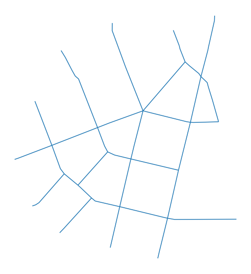
The model situation expects to have all input data for analysis in GeoDataFrames, including street network (e.g. from shapefile).
[1]:
import momepy
import geopandas as gpd
import matplotlib.pyplot as plt
import networkx as nx
[2]:
streets = gpd.read_file(momepy.datasets.get_path('bubenec'), layer='streets')
[3]:
f, ax = plt.subplots(figsize=(10, 10))
streets.plot(ax=ax)
ax.set_axis_off()
plt.show()
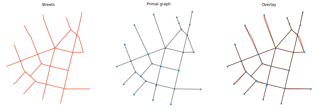
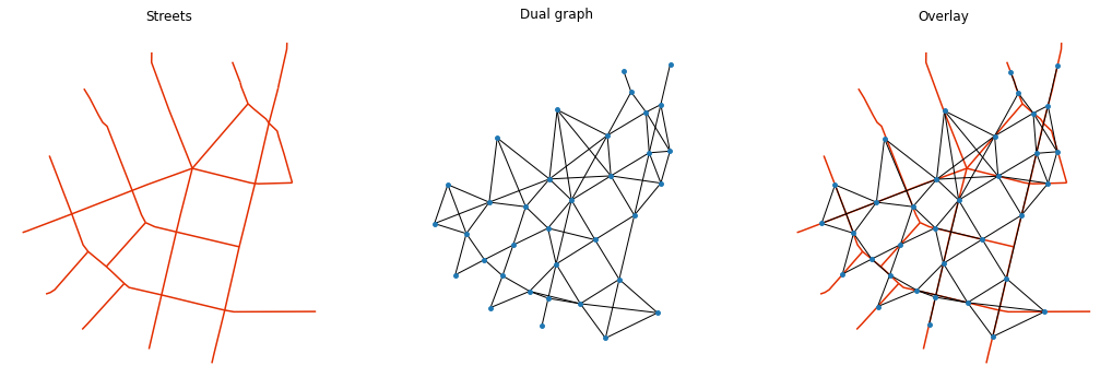
We have to convert this LineString GeoDataFrame to a networkx.Graph. We use momepy.gdf_to_nx and later momepy.nx_to_gdf as a pair of interconnected functions. gdf_to_nx supports both primal and dual graphs. The primal approach will save the length of each segment to be used as a weight later, while dual will save the angle between segments (allowing angular centrality).
[4]:
graph = momepy.gdf_to_nx(streets, approach='primal')
[14]:
f, ax = plt.subplots(1, 3, figsize=(18, 6), sharex=True, sharey=True)
streets.plot(color='#e32e00', ax=ax[0])
for i, facet in enumerate(ax):
    facet.set_title(("Streets", "Primal graph", "Overlay")[i])
    facet.axis("off")
nx.draw(graph, {n:[n[0], n[1]] for n in list(graph.nodes)}, ax=ax[1], node_size=15)
streets.plot(color='#e32e00', ax=ax[2], zorder=-1)
nx.draw(graph, {n:[n[0], n[1]] for n in list(graph.nodes)}, ax=ax[2], node_size=15)
[6]:
dual = momepy.gdf_to_nx(streets, approach='dual')
[16]:
f, ax = plt.subplots(1, 3, figsize=(18, 6), sharex=True, sharey=True)
streets.plot(color='#e32e00', ax=ax[0])
for i, facet in enumerate(ax):
    facet.set_title(("Streets", "Dual graph", "Overlay")[i])
    facet.axis("off")
nx.draw(dual, {n:[n[0], n[1]] for n in list(dual.nodes)}, ax=ax[1], node_size=15)
streets.plot(color='#e32e00', ax=ax[2], zorder=-1)
nx.draw(dual, {n:[n[0], n[1]] for n in list(dual.nodes)}, ax=ax[2], node_size=15)
At this moment (almost) any networkx method can be used. For illustration, we will measure the node degree. Using networkx, we can do:
[7]:
degree = dict(nx.degree(graph))
nx.set_node_attributes(graph, degree, 'degree')
However, node degree is implemented in momepy so we can use directly:
[8]:
graph = momepy.node_degree(graph, name='degree')
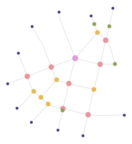
Once we have finished our network-based analysis, we want to convert the graph back to a geodataframe. For that, we will use momepy.nx_to_gdf, which gives us several options of what to export.
linesoriginal LineString geodataframe
pointspoint geometry representing street network intersections (nodes of primal graph)
spatial_weightsspatial weights for nodes capturing their relationship within a network
Moreover, edges will contain node_start and node_end columns capturing the ID of both nodes at its ends.
[9]:
nodes, edges, sw = momepy.nx_to_gdf(graph, points=True, lines=True,
                                    spatial_weights=True)
[10]:
f, ax = plt.subplots(figsize=(10, 10))
nodes.plot(ax=ax, column='degree', cmap='tab20b', markersize=(nodes['degree'] * 100), zorder=2)
edges.plot(ax=ax, color='lightgrey', zorder=1)
ax.set_axis_off()
plt.show()
[11]:
nodes.head(3)
[11]:
| degree | nodeID | geometry | |
|---|---|---|---|
| 0 | 3 | 1 | POINT (1603585.640 6464428.774) |
| 1 | 5 | 2 | POINT (1603413.206 6464228.730) |
| 2 | 3 | 3 | POINT (1603268.502 6464060.781) |
[12]:
edges.head(3)
[12]:
| geometry | mm_len | node_start | node_end | |
|---|---|---|---|---|
| 0 | LINESTRING (1603585.640 6464428.774, 1603413.2... | 264.103950 | 1 | 2 |
| 1 | LINESTRING (1603561.740 6464494.467, 1603564.6... | 70.020202 | 1 | 9 |
| 2 | LINESTRING (1603585.640 6464428.774, 1603603.0... | 88.924305 | 1 | 7 |