Proximity bands
Proximity bands are street-based morphological elements following the pedestrian perspective of urban fabric analysis described by Araldi and Fusco [2019]. Instead of representing the city from parcels, blocks, or buildings, they describe the portion of space assigned to each street segment within a fixed walking-side distance.
In momepy, momepy.proximity_bands builds these elements as a Voronoi partition of the area within a buffer around street geometry. The result is useful when a character should be measured from the street, for example the built form or land cover that can be associated with a pedestrian moving along a street segment.
The distance is expressed in the units of the CRS, so the input should use a projected CRS.
import geopandas as gpd
import mapclassify
import momepy
path = momepy.datasets.get_path("bubenec")
streets = gpd.read_file(path, layer="streets")
We start with street centerlines. The Bubenec sample data are already projected in meters.
ax = streets.plot(color="black", linewidth=2, figsize=(8, 8))
ax.set_axis_off()
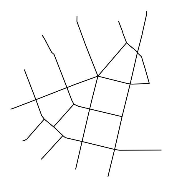
A standard proximity band assigns the area within band distance to the nearest street segment. Here, each segment gets one polygon, clipped to a 20 metre buffer around the street network.
bands = momepy.proximity_bands(streets, band=20)
bands.head()
| geometry | |
|---|---|
| 0 | POLYGON ((1603419.57 6464266.746, 1603562.598 ... |
| 1 | POLYGON ((1603268.523 6464060.801, 1603282.94 ... |
| 2 | POLYGON ((1603413.18 6464228.695, 1603413.178 ... |
| 3 | POLYGON ((1603640.25 6464408.422, 1603640.262 ... |
| 4 | POLYGON ((1603542.571 6464488.589, 1603539.027... |
unique_color = mapclassify.greedy(bands)
ax = bands.plot(
    unique_color,
    categorical=True,
    edgecolor="white",
    linewidth=0.4,
    figsize=(8, 8),
)
streets.plot(ax=ax, color="black", linewidth=1)
ax.set_axis_off()
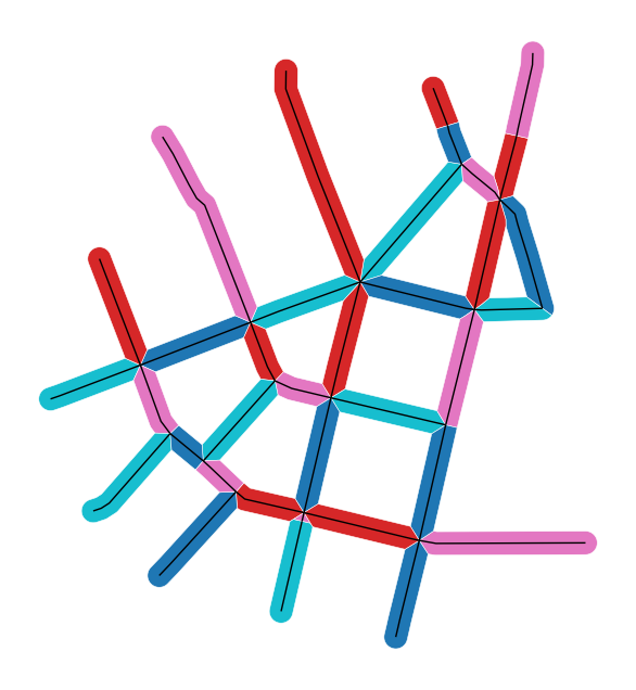
The default output has the same index as the input streets, which makes it straightforward to attach measurements back to street segments.
bands.index.equals(streets.index)
True
Single-sided bands
Araldi and Fusco’s pedestrian perspective treats the street as the observation axis. In many situations, the two sides of a street expose different urban fabric: buildings, plots, or open space may differ across the centerline. Passing single_sided=True splits the band along the street geometry and returns separate polygons for each side.
single_sided = momepy.proximity_bands(streets, band=20, single_sided=True)
single_sided.head()
| geometry | |
|---|---|
| 0 | POLYGON ((1603419.57 6464266.746, 1603562.598 ... |
| 1 | POLYGON ((1603585.622 6464428.769, 1603562.598... |
| 2 | POLYGON ((1603585.623 6464428.754, 1603585.622... |
| 3 | POLYGON ((1603585.623 6464428.754, 1603587.435... |
| 4 | POLYGON ((1603587.435 6464400.208, 1603585.623... |
unique_color = mapclassify.greedy(single_sided)
ax = single_sided.plot(
    unique_color,
    categorical=True,
    edgecolor="white",
    linewidth=0.4,
    figsize=(8, 8),
)
streets.plot(ax=ax, color="black", linewidth=1)
ax.set_axis_off()
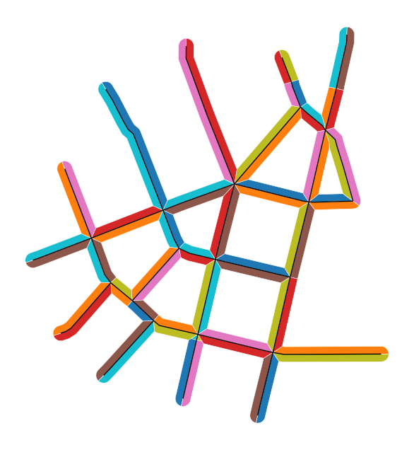
Use the two-sided version when every street segment should be represented by one element. Use the single-sided version when the analysis needs to distinguish the left and right sides of the pedestrian environment.