Note
Measuring diversity
As important diversity is for cities, as complicated is to capture it. momepy offers several options on how to do that using urban morphometrics. Generally, we can distinguish three types of diversity characters, based on:
Absolute values
Relative values
Categorization (binning)
This notebook provides examples from each of them.
[1]:
import momepy
import geopandas as gpd
import matplotlib.pyplot as plt
We will again use osmnx to get the data for our example and after preprocessing of building layer will generate tessellation.
[2]:
import osmnx as ox

gdf = ox.geometries.geometries_from_place('Kahla, Germany', tags={'building':True})
gdf_projected = ox.projection.project_gdf(gdf)

buildings = momepy.preprocess(gdf_projected, size=30,
                              compactness=True, islands=True)
buildings['uID'] = momepy.unique_id(buildings)
limit = momepy.buffered_limit(buildings)
tessellation = momepy.Tessellation(buildings, unique_id='uID', limit=limit).tessellation
Loop 1 out of 2.
Identifying changes: 100%|██████████| 2932/2932 [00:00<00:00, 7106.34it/s]
Changing geometry: 100%|██████████| 630/630 [00:04<00:00, 152.46it/s]
Loop 2 out of 2.
Identifying changes: 100%|██████████| 2115/2115 [00:00<00:00, 16914.35it/s]
Changing geometry: 100%|██████████| 172/172 [00:01<00:00, 170.48it/s]
Inward offset...
Discretization...
6%|▌ | 111/2008 [00:00<00:01, 1109.29it/s]
Generating input point array...
100%|██████████| 2008/2008 [00:01<00:00, 1824.22it/s]
Generating Voronoi diagram...
Generating GeoDataFrame...
Vertices to Polygons: 100%|██████████| 249298/249298 [00:04<00:00, 54255.22it/s]
Dissolving Voronoi polygons...
Preparing limit for edge resolving...
Building R-tree...
Identifying edge cells...
Cutting...
0it [00:00, ?it/s]
Queen contiguity
Morphological tessellation allows using contiguity-based weights matrix. While libpysal.weights.contiguity.Queen will do a classic Queen contiguity matrix; it might not be enough to capture proper context. For that reason, we can use momepy.sw_high to capture all neighbours within set topological distance k. More in Generating spatial weights.
[3]:
sw3 = momepy.sw_high(k=3, gdf=tessellation, ids='uID')
To have a character whose diversity can be measured, we can use the area of tessellation.
[4]:
tessellation['area'] = momepy.Area(tessellation).series
Range
The range is as simple as it sounds; it measures the range of the values withing all neighbours as captured by spatial_weights.
[5]:
area_rng = momepy.Range(tessellation, values='area',
                                        spatial_weights=sw3, unique_id='uID')
tessellation['area_rng'] = area_rng.series
100%|██████████| 2005/2005 [00:00<00:00, 2617.70it/s]
[6]:
f, ax = plt.subplots(figsize=(10, 10))
tessellation.plot(ax=ax, column='area_rng', legend=True, cmap='Spectral_r')
buildings.plot(ax=ax, color="white", alpha=0.4)
ax.set_axis_off()
plt.show()
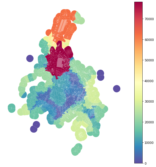
However, as we can see from the plot above, there is a massive effect of large-scale buildings, which can be seen as outliers. For that reason, we can define rng keyword argument to limit the range taken into account. To get the interquartile range:
[7]:
area_iqr = momepy.Range(tessellation, values='area',
                        spatial_weights=sw3, unique_id='uID',
                        rng=(25, 75))
tessellation['area_IQR'] = area_iqr.series
100%|██████████| 2005/2005 [00:00<00:00, 2467.33it/s]
[8]:
f, ax = plt.subplots(figsize=(10, 10))
tessellation.plot(ax=ax, column='area_IQR', legend=True, cmap='Spectral_r')
buildings.plot(ax=ax, color="white", alpha=0.4)
ax.set_axis_off()
plt.show()
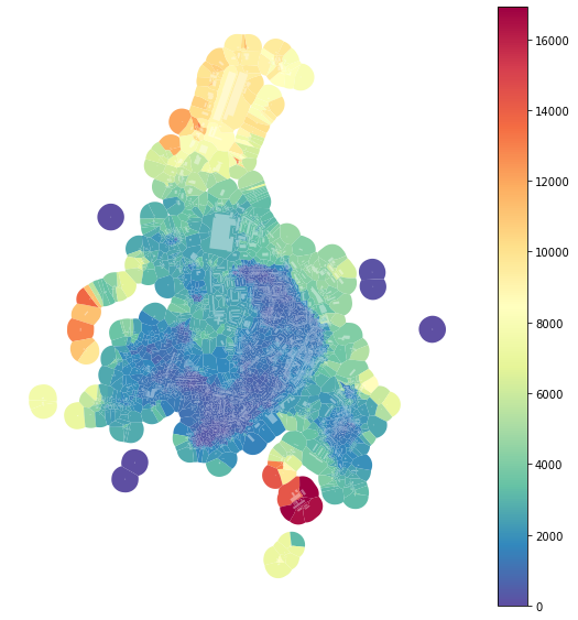
The effect of outliers has been successfully eliminated.
Theil index
Theil index is a measure of inequality (as Gini index is). momepy is using pysal’s implementation of the Theil index to do the calculation.
[9]:
area_theil = momepy.Theil(tessellation, values='area',
                          spatial_weights=sw3,
                          unique_id='uID')
tessellation['area_Theil'] = area_theil.series
100%|██████████| 2005/2005 [00:01<00:00, 1099.79it/s]
[10]:
f, ax = plt.subplots(figsize=(10, 10))
tessellation.plot(ax=ax, column='area_Theil', scheme='fisherjenks', k=10, legend=True, cmap='plasma')
buildings.plot(ax=ax, color="white", alpha=0.4)
ax.set_axis_off()
plt.show()
Again, the outlier effect is present. We can use the same keyword as above to limit it and measure the Theil index on the inter-decile range.
[11]:
area_id_theil = momepy.Theil(tessellation, values='area',
                             spatial_weights=sw3,
                             unique_id='uID',
                             rng=(10, 90))
tessellation['area_Theil_ID'] = area_id_theil.series
100%|██████████| 2005/2005 [00:00<00:00, 2071.59it/s]
[12]:
f, ax = plt.subplots(figsize=(10, 10))
tessellation.plot(ax=ax, column='area_Theil_ID', scheme='fisherjenks', k=10, legend=True, cmap='plasma')
buildings.plot(ax=ax, color="white", alpha=0.4)
ax.set_axis_off()
plt.show()
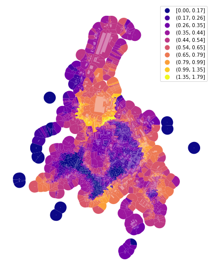
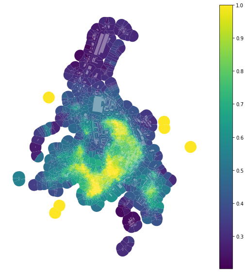
Simpson’s diversity index
Simpson’s diversity index is one of the most used indices capturing diversity. However, we need to be careful using it for continuous values, as it depends on the binning of these values to categories. The effect of different binning could be significant. momepy uses Head/tail Breaks as a large number of morphometric characters follows power-law distribution (for which Head/tail Breaks are designed). However, you can use any binning provided by mapclassify (including user-defined). The
default Head/tail Breaks:
[13]:
area_simpson = momepy.Simpson(tessellation, values='area',
                              spatial_weights=sw3,
                              unique_id='uID')
tessellation['area_simpson'] = area_simpson.series
 10%|█         | 208/2005 [00:00<00:03, 488.39it/s]/opt/miniconda3/envs/momepy_guide/lib/python3.8/site-packages/mapclassify/classifiers.py:888: RuntimeWarning: invalid value encountered in double_scalars
  gadf = 1 - self.adcm / adam
100%|██████████| 2005/2005 [00:02<00:00, 932.39it/s]
[14]:
f, ax = plt.subplots(figsize=(10, 10))
tessellation.plot(ax=ax, column='area_simpson', legend=True, cmap='viridis')
buildings.plot(ax=ax, color="white", alpha=0.4)
ax.set_axis_off()
plt.show()
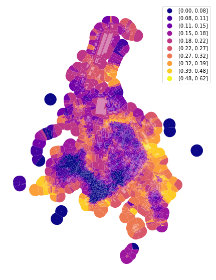
And binning based on quantiles (into 7 bins of equal size):
[15]:
tessellation['area_simpson_q7'] = momepy.Simpson(tessellation, values='area',
                                                 spatial_weights=sw3,
                                                 unique_id='uID',
                                                 binning='quantiles', k=7).series
  7%|▋         | 131/2005 [00:00<00:01, 1302.73it/s]/opt/miniconda3/envs/momepy_guide/lib/python3.8/site-packages/mapclassify/classifiers.py:888: RuntimeWarning: invalid value encountered in double_scalars
  gadf = 1 - self.adcm / adam
100%|██████████| 2005/2005 [00:01<00:00, 1157.35it/s]
[16]:
f, ax = plt.subplots(figsize=(10, 10))
tessellation.plot(ax=ax, column='area_simpson_q7', legend=True, cmap='viridis')
buildings.plot(ax=ax, color="white", alpha=0.4)
ax.set_axis_off()
plt.show()
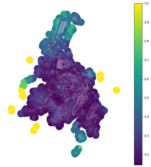
Always consider whether your binning is the optimal one.